BUDGETING TIP OF THE MONTH

Pivot Table Tips for Importing Data

 

Do you have trouble manipulating data to get it into a format that can be easily copied into a template for importing purposes, particularly when using a pivot table? Often, if you are unfamiliar with some of the features of pivot tables, it can be a grueling experience to get data into a format that is easily copied into an import template.

Here are a few tips to help improve efficiency!

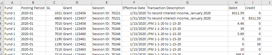
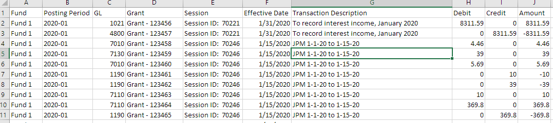
Below is a sample of raw data that we would like to summarize by period (effective date) and various dimensions/segments including GL to copy into a template for importing purposes.

 

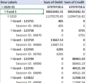
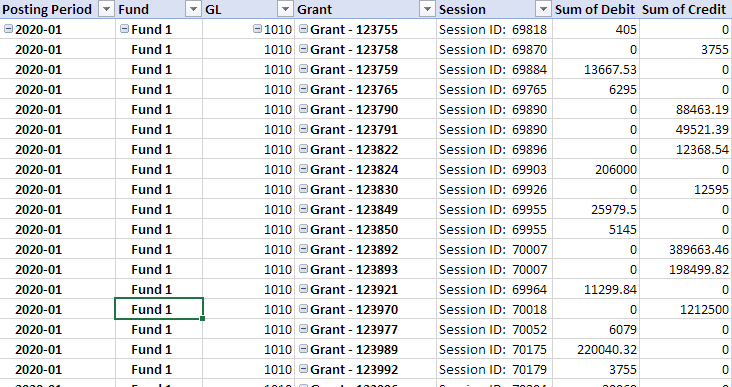
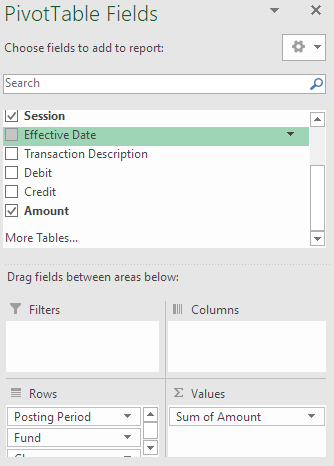
Without knowing some key features of pivot tables, you might create a pivot table that looks like this and will require a lot of manipulation to get it into a format that can easily be copied into your template. Here we’ve selected the Posting Period, Fund, GL, and Grant for the Rows, then added our Values of Debit and Credit.

 

You may have been trying to copy and paste this information into another sheet and then copying headers to fill in the blanks on rows to get it into a format that is sufficient for your import template and removing subtotals. There is a quicker, easier way!

First, you’ll notice a menu grouping in Excel for PivotTable Tools and the selection of Analyze or Design.

 

Select the Design option, and under Subtotals, select the option “Do not show subtotals’ to remove all subtotals.

Next, under Grand Totals, select the option “Off for Rows and Columns”.

Then from the Report Layout menu, select the option “Show in tabular form”. Your pivot table should look something like this:

 

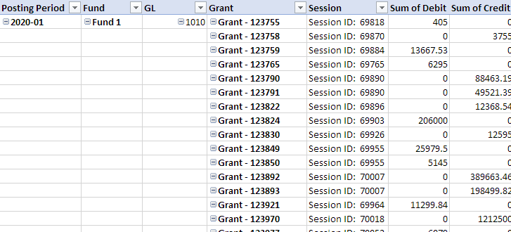
But now we have the issue of blank cells where we would like the labels included to make it easier to copy and paste into our template. To remedy this, select Report Layout option again and then select the option "Repeat all item labels.” Now, your pivot table should look something like this:

 

While the pivot table is now in a format that can easily be copied into your import template, there are a couple more options you may want to consider.

First, on the Analyze option from the PivotTable Tools menu, the +/- Buttons option is selected by default. Click this option to ‘de-select’ it. This will remove the options from the pivot table.

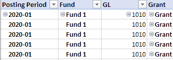
Before with the +/- Buttons default:

 

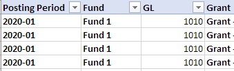
After removing +/- Buttons:

 

You may consider consolidating your values into one column. This requires going back to your raw data and inserting a column and using formulas to consolidate the data into one column, being mindful of the sign of the value required for your system and natural account’s normal balance.

 

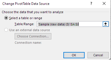
Next, you’ll need to expand your pivot table to include the new column. To do this, select Change Data Source from the Analyze, PivotTable Tools menu, and select all the data you need for your pivot table.

 

Then refresh your pivot table by selecting the Refresh option on the Analyze menu. Remove the Debit and Credit options from the Values field of the Pivot table and replace them with your consolidated data column.

 

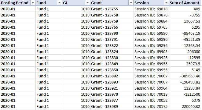
Finally, your pivot table should look something like this and be ready to copy and paste into your import template.